GROMACS tutorial 3: Several methanes in water

In this tutorial, I'll show you how to create a system containing several OPLS methane in a box of TIP4PEW water and get the methane-methane potential of mean force from this information.

Setup

Reuse methane.pdb and topol.top from the last tutorial (make copies). Remove all of the waters in topol.top by deleting the line containing SOL under [ molecules ]. We're going to perform our simulation on 10 methanes in 1000 waters. As a starting point, we'll set the box to be 3.2 nm in each direction. Obviously, when we add pressure coupling this will go to the correct size, but we want to start somewhere close. The density of water is close to 33.5 molecules / nm^3, so the cube root of 1010/33.5 is around 3.11, so rounding up gives me 3.2 nm.

First, insert ten methanes into a 3.2 nm x 3.2 nm x 3.2 nm box:

$ gmx insert-molecules -ci methane.pdb -o box.gro -nmol 10 -box 3.2 3.2 3.2

Update the line in topol.top containing the number of methanes from 1 to 10.

Then add water to the box:

$ gmx solvate -cs tip4p -cp box.gro -o conf.gro -p topol.top -maxsol 1000

The command gmx solvate automatically updates topol.top for us.

Reuse the .mdp files from last time, except change nsteps in prd.mdp to be longer. I myself ran this for 100 ns, so I simply added a 0 to the end of the number from last time. You may also want to output more frequently for our analysis below.

Simulation

Run the simulation just like last time.

Analysis

Create an index file containing a group of the 10 methanes:

$ gmx make_ndx -f conf.gro

> a C
> q

Now use gmx rdf just like last time, but instead choose the group containing C twice.

Depending on how many frames you saved and how long you ran the simulation (I ran mine for 100 ns and saved 25,000 frames), you should get an RDF that looks something like this if you just plot it normally:

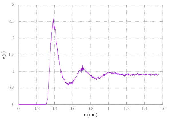
Note that it does not converge to one. We are overcounting by one, so we should factor that out. Here's the gnuplot command:

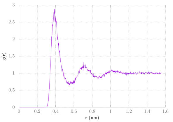
> plot 'rdf.xvg' u 1:($2*10/9) w l

We have ten methanes, but we should only be counting nine with the RDF, so we multiply the value of g by N/(N-1), which is 10/9. It should look like this:

Now to get the methane-methane potential of mean force (PMF) from the methane-methane RDF we do w = -kTln(g).

So to plot this with gnuplot do:

> plot 'rdf.xvg' u 1:(-8.314e-3*298.15*log($2*10/9)) w l

Your plot should look something like this:

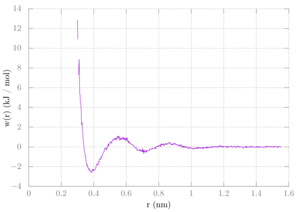
You notice there is a small gap in our sampling. The methanes never interacted at that distance. We'll use umbrella sampling in a later tutorial to solve this.

Summary

In this tutorial, we created a box of 10 methanes and 1000 waters using gmx insert-molecules and gmx solvate. We simulated this just like last time, except we did it a little longer. We again used gmx rdf to get the radial distribution function, but this time for methane-methane. We had to add a correction due to this, and from there we were able to get the potential of mean force.

Author: Wes Barnett, Vedran Miletić